OCT choriocapillaris flow deficits quantification software Manual
Version 1.2
Table of Contents
1. Introduction
This software provides an easy graphical user interface (GUI), based on python, to read and write a wide range of OCT/OCTA image data, perform segmentation, visualize 3D images, and write processed datasets for choriocapillaris flow deficits. It also contains high efficient image processing algorithms.
2. Installation
2.1 Create a folder of your choice, and copy the zipped files as provided into this folder.
2.2 Check your computer settings. The software requires ffmpeg, elastix to properly run. If these are not available in your computer, do not worry. Double click the ‘setup.bat’ file provided in the package to set up these dependences.
2.3 Unzip the package and run the main.exe. You are good to go!
3. Requirements of computer
Operation system: Windows 7/10
Memory: >16GB
Free disk space: >10GB
CPU: 4 cores 4.0 GHz (segmentation process for 1200x500x500 images, ~3minutes)
2 cores 3.2 GHz (segmentation process for 1200x500x500 images, ~5minutes)
4. Overview
The layout of the user interfaces is shown in the figures below. These are 2 main windows for image visualization and manual segmentation correction.
Description of the modules:
3.1 This is the main window of the software. It allows user to load, display, segment the OCT 3D volume as well as to generate, display and save en face images of selected slabs.
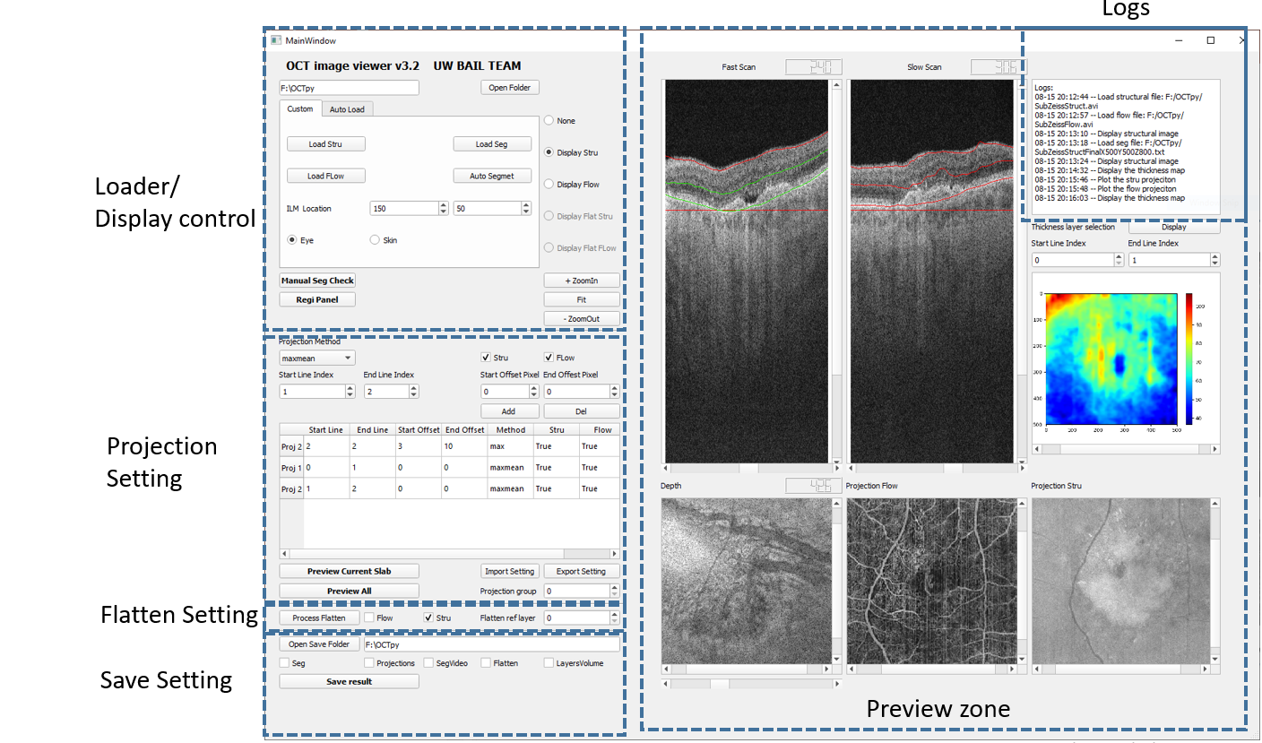
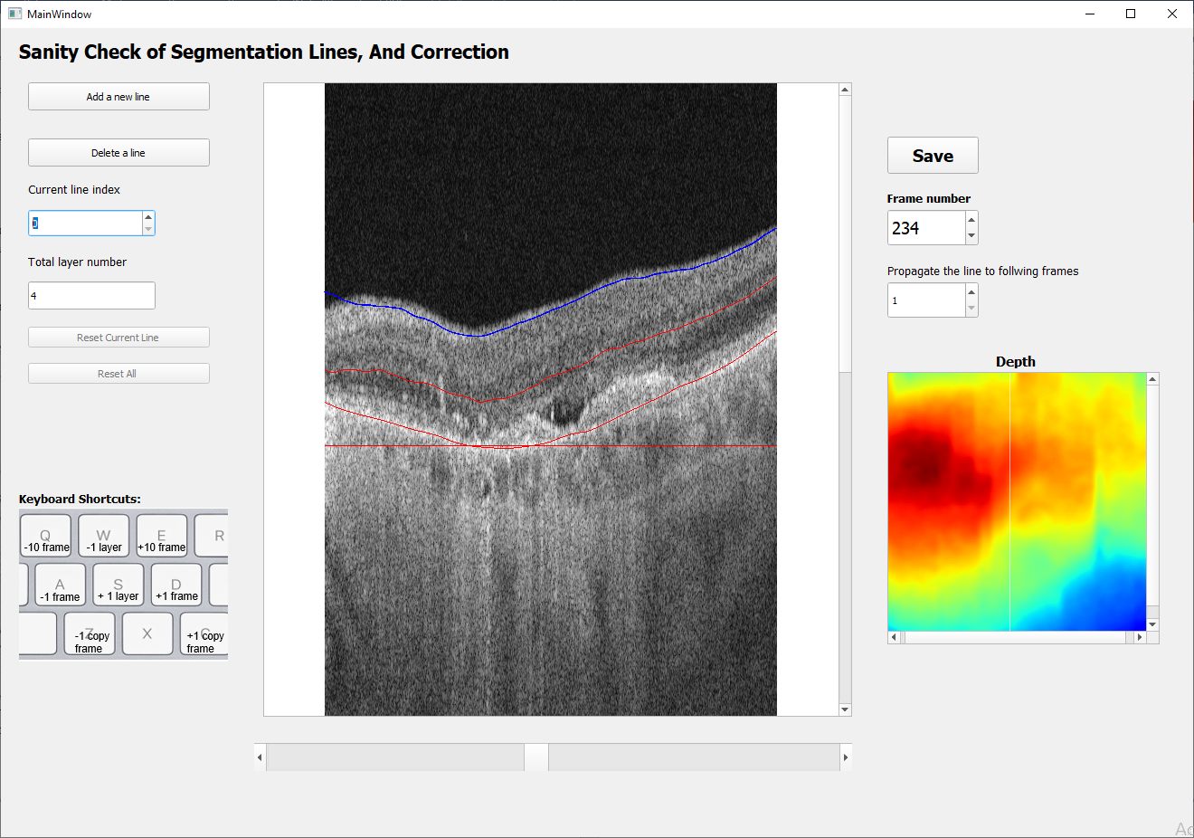
3.2 This window allows for visualization of automatic segmentation lines and manual correction if necessary.
5. Usage
This software has following features:
-
Load videos and display OCT, OCTA 3D data.
-
Automatic segmentation of loaded data.
-
Manual correction of incorrect auto-segmentation lines.
-
Define desired slabs and generate en face images.
-
Segment choriocapillaris flow deficits and perform quantification.
-
Save all processed results
-
Batch processing
4. Overview and the procedures to use the software
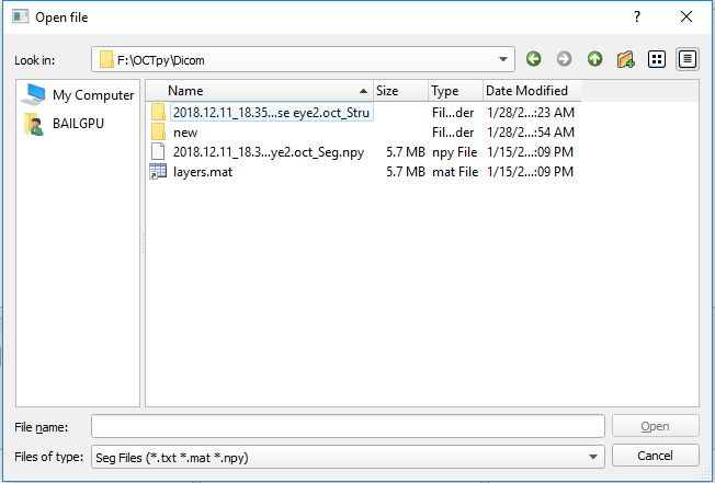
4.1 Image loader
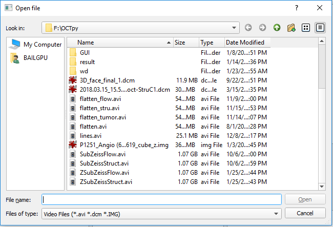
• Select the files path
• Load structural volume
• Load flow volume
• Load manual segmentation file/Run auto segmentation
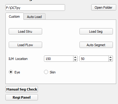
To load the OCT and OCTA data files, use the ‘Load Stru’ and ‘Load Flow’ buttons respectively. Supported formats include: avi, Zeiss img, and dicom.
If the segmentation files are already available, use the ‘Load Seg’ button to load files with npy, mat and txt formats. If segmentation files are not available, click the button ‘Auto Segment’ to perform automatic segmentation. The progress is displayed in a separate command line window. The current software will segment 4 lines: ILM, RPE, RPE-fit and BM (required to have both the structural and flow data). You need load the structural and flow data before performing the segmentation.

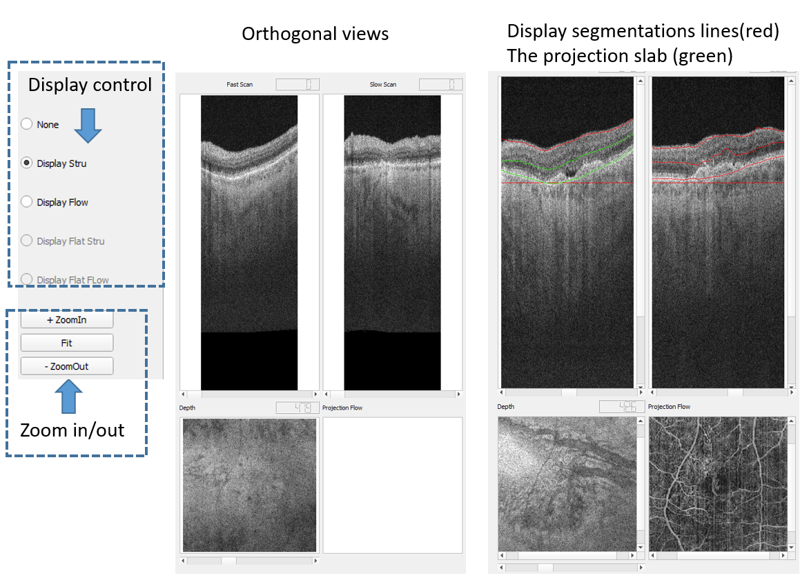
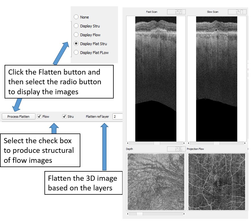
4.2 3D image display
After loading videos into the workspace, the radio buttons are enabled for displaying the 3D volumes. Three separate windows display the slice of fast scan, slow scan, and the depth en face view. Toggle the scroll bar to change the slice of display. If the segmentation file is loaded (see right figure), the red lines present the results of segmentation and the green lines show the custom slab for the visualization of en face projection of this slab.
4.3 Image segmentation
4.3.1 Auto segmentation
Auto-segmentation of the ILM, RPE, RPE-fit and BM are achieved by clicking the ‘Auto Segment’ button. Visualization of the segmentation lines could be achieved by either displaying 3D data as described in 4.2, or by going in to the manual correction view by clicking the ‘Manual Correct’ button.
4.4 Manual Correction of Segmentation Lines
To make manual corrections on automatic segmentation lines, user can click the ‘Manual Correct’ button to open the Segmentation Window. Users can edit segmentation lines frame by frame and add new lines.
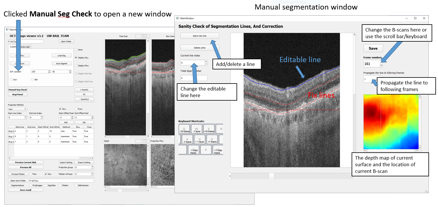
To use the manual segmentation tool, select the line that user wants to change (blue), left click the mouse and draw the line to the new location.
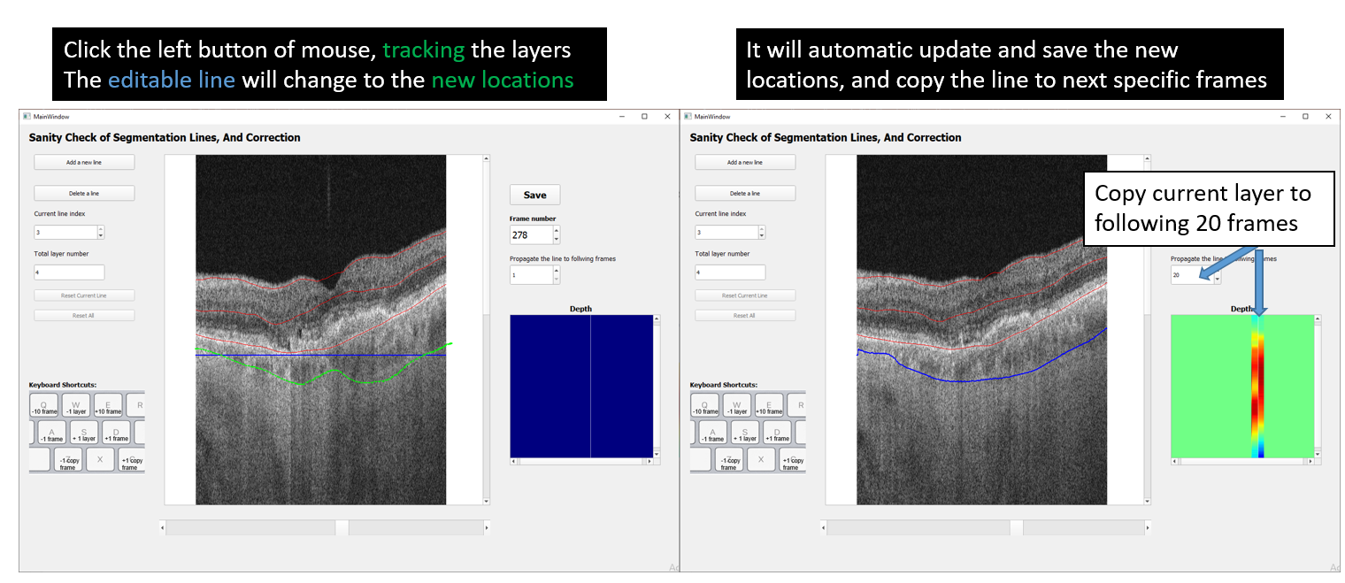
After correcting segmentation lines of selected B-scans, updated segmentation files can be saved by clicking the Save button as shown in the figure above.
keyboard shortcuts:
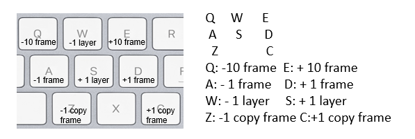
Shift: display/ not display the lines
4.5 Generate En face Projections
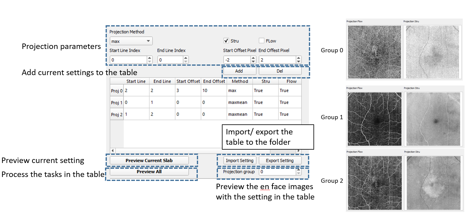
To obtain en face projection of desired slabs, users can set the parameters in the panel with following procedures.
- Adjust the parameters in the panel for slab definition; the defined slab is displayed on the fast scan window between green lines.
-
Use the ‘Add’ button to add the parameters to the table.
-
Repeat 1&2 to add multiple slabs.
-
Click the button Preview Current Slab to preview the results.
-
Toggle the spin box of Preview all to review different slabs.

-
Select the row in the table and click the ‘Del’ button to remove the unwanted results.
-
Use the ‘Export setting’ button to save the projection setting. Next time, the user can import this this saved csv file by ‘Import Setting’ to configure the same settings.
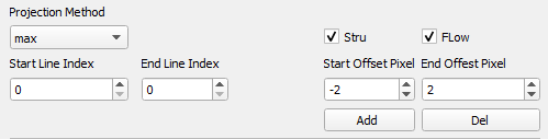
Explanation of projection parameters:
• Projection method: MIP (maximum intensity projection), sum (sum projection), min (minimum intensity projection), etc.
• Start line: The index of the lines of upper boundary
• End line: The index of the line of lower boundary
• Start offset: The offsets of the upper boundary, positive value to move down, negative to move up (in pixels)
• End offset: The offsets of the lower boundary, positive value to move down, negative to move up (in pixels)
• Preview: Display the en face projection using current settings
• Add/ del: add or delete current settings to the table and saving
• Proj All: Process all projections in the table
To generate proper CC slab, we recommend settings as below,
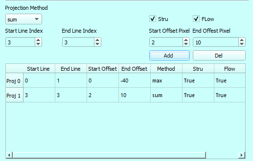
The fist slab defines the retinal layer and the second layer defines the CC layer.
4.6 Flatten the volume based on segmentation lines
The user can specify a reference segmentation line to flat the 3D volume. This function can be enabled after the segmentation is done, or if there are segmentation files available.
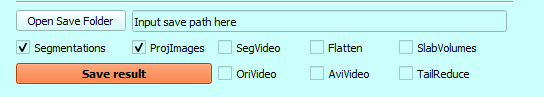
4.7 Save the Results
\1. Click the button ‘Open Save Folder’ or input the path to the window.
\2. Select the check box of files to save
\3. To generate the CC slab, select the ‘Segmentations’ and ‘ProjImages’
And then click the button ‘Save Result’.
The following files will be saved in the designated folder,
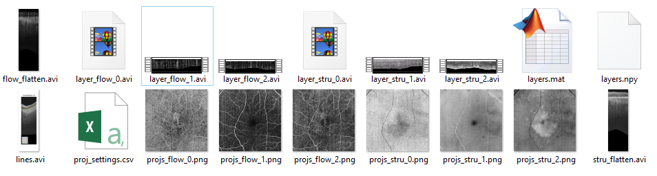
• layers.mat/ layers.npy save the segmentation lines information.
• Lines.avi: visually display the results of segmentation lines.
• Porj_setting.csv: the parameters for projection, can be further used for batch processing
• Projs_.png: *en face projection images
• *_flatten.avi: The flattened videos
• Layer_*_num.avi: the slab volumes
4.8 Batch processing
All process above (4.1-4.7) could be automated with batch processing mode.
To use it, select the tab ‘Auto Load’ to start with. The software will detect the files in the same folder with custom defined rules. It will load the 3D volumes and make the en face projections based on the parameters defined in the main window. If the segmentation files do not exist in the folder, it will perform auto-segmentation on loaded volumes.
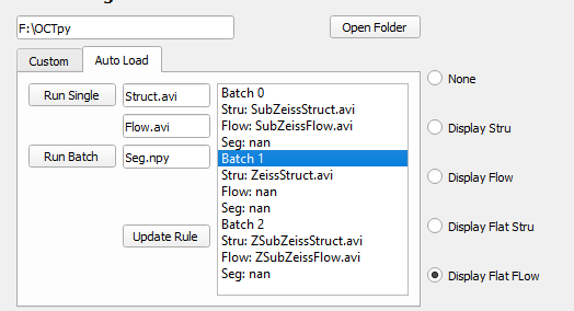
Steps to use the batch processing mode:
-
Define the rules of filename, files with names containing the same ending will be automatically detected.
-
Select the folder that contains the video and segmentation files by clicking “Open Folder”.
-
Check the saving/projection setting before click the ‘Run’ button.
-
Click the ‘Run Batch’ button to process all listed files or select single file on the list and click the ‘Run Single’ button to process.
4.9 the CC quantification tool
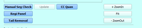
Open the tool
Open the CC quantification tool from the main panel by clicking the ‘CC quan’ button. This tool accepts input images of OCTA CC image, OCT CC image and OCTA retina image. It performs OCTA CC compensation using OCT CC image, OCTA CC projection artifacts removal using OCTA retina image, and CC flow deficits quantification using compensated, projection artifacts removed OCTA CC image.
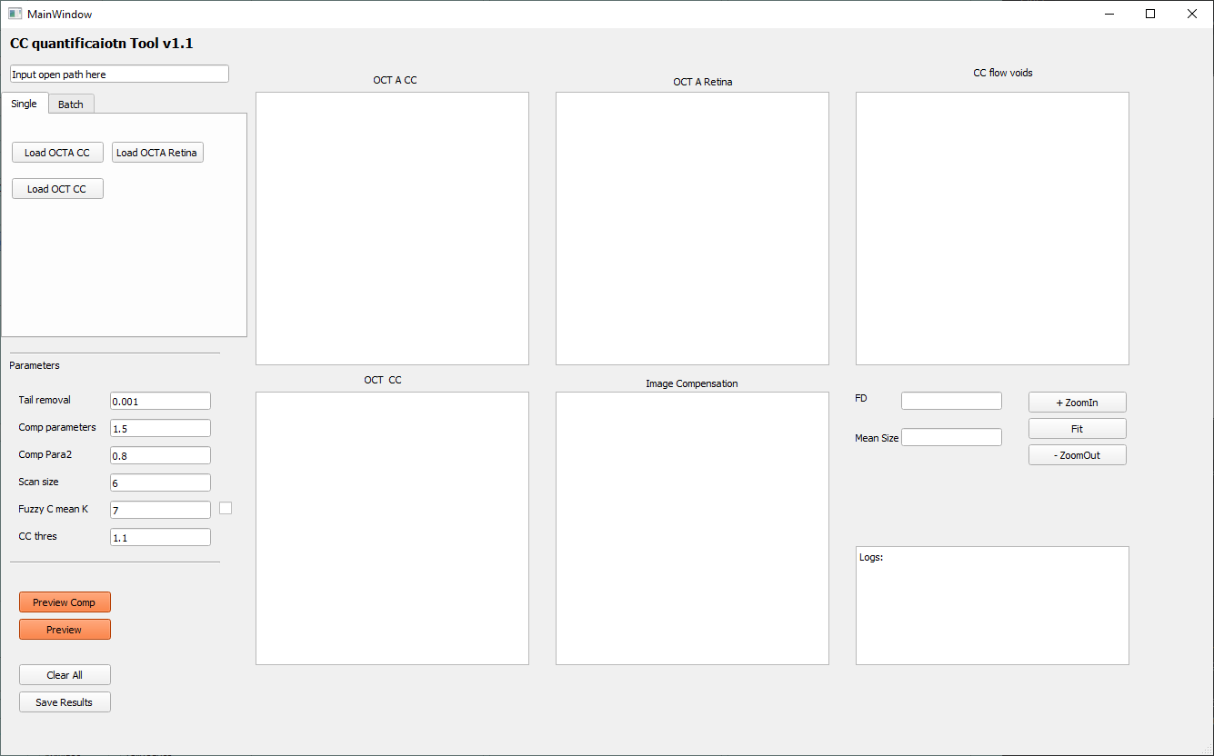
Single mode
To load the specific images to quantifying the flow deficits, click the ‘load OCTA CC’, ’load OCTA Retina’, ‘load OCT CC’ button on by one. If you used previous projection setting, these files are:
‘porjs_flow_1.png’, ‘projs_flow_0.png’, ‘projs_stru_1.png’
Batch mode
Add the file name rules to the batch processing tab.
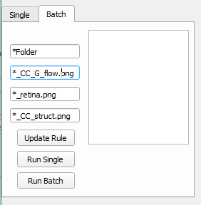
Put the pattern of file folder name, OCTA CC image, ’load OCTA Retina’, ‘load OCT CC’ to the text editors. The * represents any characters. Then click ‘Update Rule’ to select the folder that contains your data. An example of data files and the name rules is presented below.
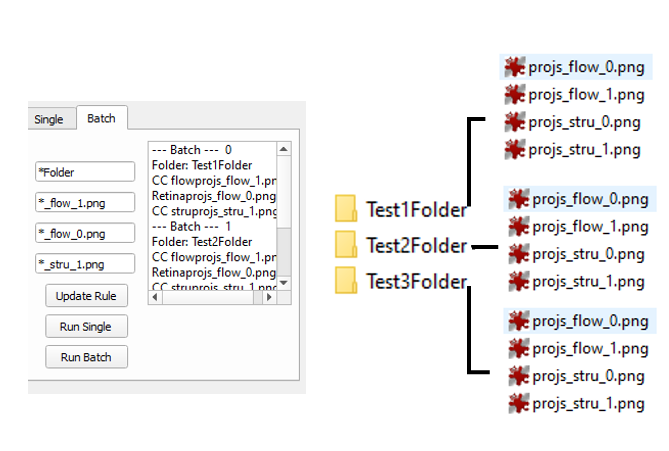
To process the data, select the file in the list and then click the Run Single. All click the Run Batch.
Adjust the parameters
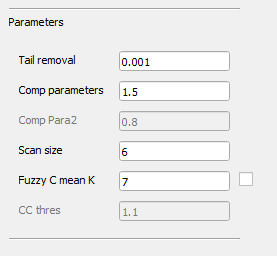
Usually, users may use the default parameters for quantification.
Tail removal: The parameter used for retinal projection artifacts removal, a larger number leads to stronger artifacts removal.
Comp parameters: The parameter used for OCTA CC compensation, a larger number leads to weaker compensation effects.
Scan size: The size of the OCTA scan.
Fuzzy C mean K: The number of memberships used for classification, this parameter is automatically calculated using the elbow method, but can be manually adjusted if desired.
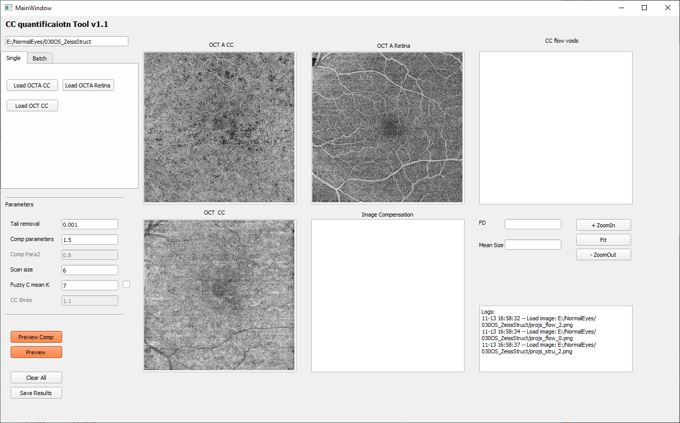
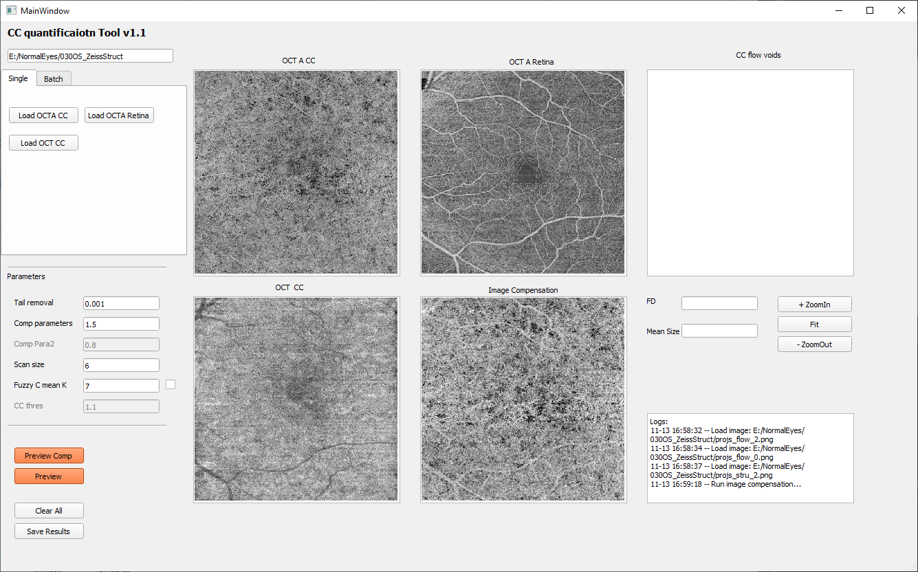
Preview compensation
The compensation process includes OCT CC structural compensation and retinal projection artifacts removal, click the ‘Preview Comp’ button to visualize processed results.
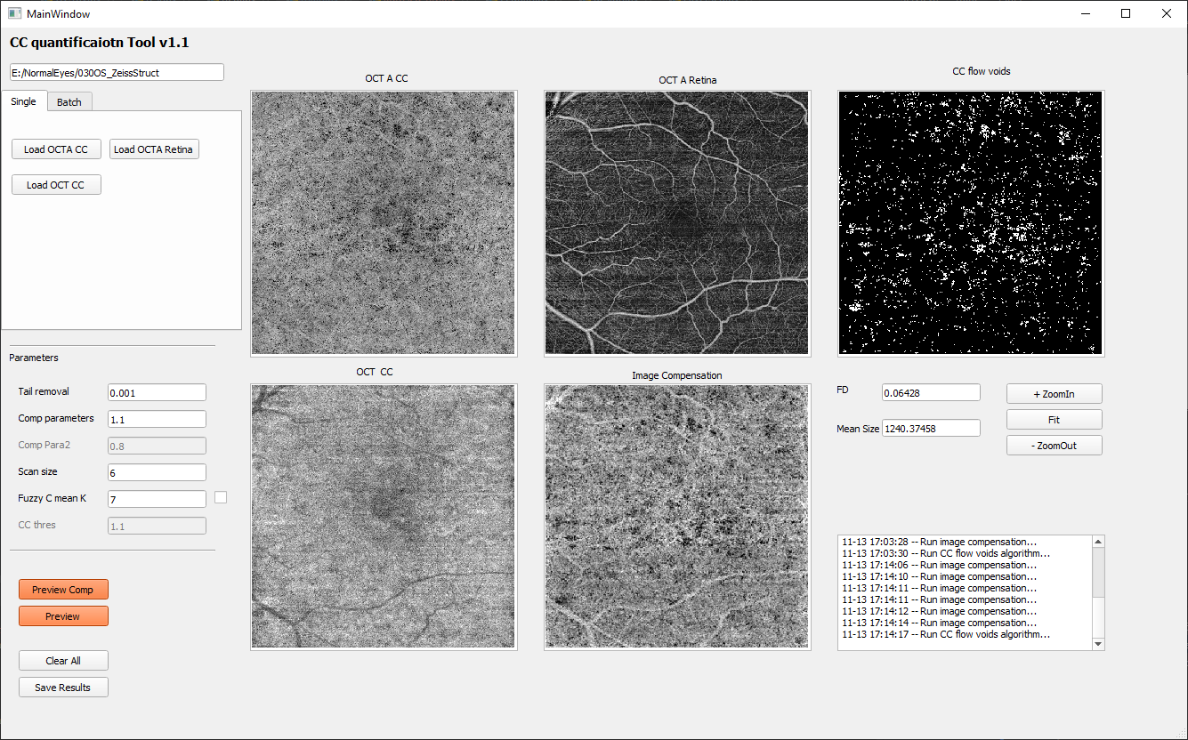
Preview quantification result
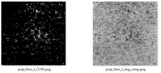
Click the ‘Preview’ button to calculate the choriocapillaris flow deficits. The numerical values of flow deficit density and mean flow deficit size (µm2) as well as the binarized flow deficits map (white pixels represents flow deficits) will be displayed on the right side as shown below. Of note, in the binarized flow deficits map, individual flow deficits with an equivalent diameter smaller than 24 µm have been removed.
Save the results
To save the results, click the ‘Save Results’ button. The program will create a new folder with the same of the image file to save the results.
Quantification results:
The file image_filename_cc_results.csv

Image results:
The binary CC flow deficits map and the CC OCTA image after compensation.
Reference:
Chu, Z., Zhou, H., Cheng, Y., Zhang, Q., & Wang, R. K. (2018). Improving visualization and quantitative assessment of choriocapillaris with swept source OCTA through registration and averaging applicable to clinical systems. Scientific reports, 8(1), 1-13.
Zhang, Q., Zheng, F., Motulsky, E. H., Gregori, G., Chu, Z., Chen, C. L., … & Wang, R. K. (2018). A novel strategy for quantifying choriocapillaris flow voids using swept-source OCT angiography. Investigative ophthalmology & visual science, 59(1), 203-211.
Zhang, A., Zhang, Q., & Wang, R. K. (2015). Minimizing projection artifacts for accurate presentation of choroidal neovascularization in OCT micro-angiography. Biomedical optics express, 6(10), 4130-4143.